Lab 3 Machine Learning & Prediction
Overview
In the previous lab we examined the practice of feature selection - identifying the proper set of variables to use as inputs into a predictive model. Gottman developed a framework using 20 micro-expressions coded at one-second intervals. Iceland developed a set of variables that help predict whether teens are likely to abuse alcohol.
A key pattern that emerges from the case studies and a take-away from Lab 2 is that identifying the proper data to include in a model is difficult. Typically, experts start with a large number of measures and eliminate variables as they are tested. It requires patience and attention to detail to identify the right set of variables for a given problem.
This week we will explore the process of “feature engineering,” the task of starting from raw data sources and “engineering” new variables by finding ways to code or extract new features. Feature engineering is common when using data like satellite imagery, document archives, or video. It is common that the data was not designed for the task at hand, but it contains rich information that is extremely valuable if it can be extracted.
Feature engineering is also necessary because predictive models typically require quantitative variables, so data sources like images and text need to be transformed into counts and scales. “Engineering” can be simple or complex. A simple example is computing a new variable, BMI, from two existing ones (height and weight). More complex examples of what this process might look like for unstructured data are below.
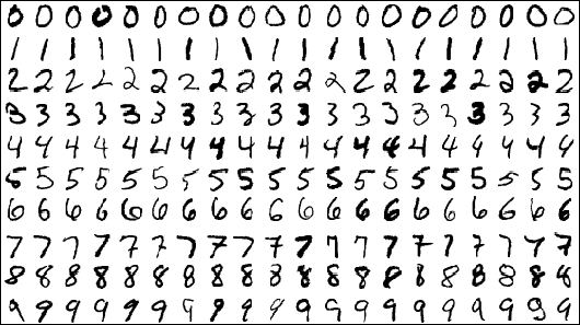
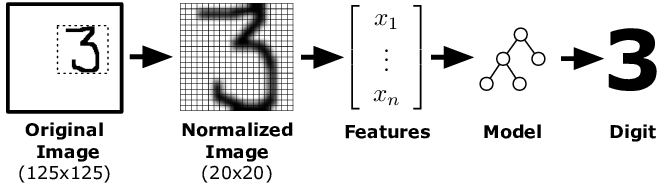
For example, how can a computer read handwriting? It has to be able to translate easily from an image of hand-written text to some sort of mathematical abstraction of the sentences.
It accomplishes this by isolating words, then isolating individual characters, then using a pixel grid to code which features exist on each character (vertical lines, curved lines, cross-bars, etc.), and making a prediction about which letter might be based upon specific features.

(Note, the elements above are concepts from typography that describe fonts, not a list of features from natural language processing, but you get the idea)
Without a set of features extracted from the raw image of a character, the computer can’t predict which letter it might be. In this way Lab 4 on Feature Engineering combines elements of Lab 2 on Measurement, and Lab 3 on Feature Selection. You “engineer” or “extract” a feature by first defining it (does the character possess a “bowl”), and then figuring out how the computer will observe or measure that feature.
The goal of this lab is to demonstrate a couple of processes of feature engineering from common machine learning and artificial intelligence applications. I would like you to develop an intuitive sense of how engineers approach the creative endeavor of turning raw data into meaningful quantitative measures. Some steps below show how raw data might be processed to make it interpretable (to code characters from text, you first need to isolate individual characters). Others steps show how raw data is translated into a quantitative variable that can be used as an input into a model.
As you read through the lab, think about the readings from Social Physics. How did computer scientists approach the task of understanding team performance in organizations? What sorts of data did they collect, and how did they generate quantitative measures from the raw data inputs of environmental sensors and employee smart badges? There are thousands of potential variables you could generate from human interactions in organizations, so how did they decide which measures were important? These themes will be revisited when we look at how Google tried to design the perfect team.
We start here with some basic examples of feature engineering in a few task domains.
Optical Character Recognition
The process by which computer programs read handwriting or scan images of text is quite interesting because of how raw image files are converted into structured data. The process is broadly called Optical Character Recognition. short video
For these tasks the program must first take an image and identify the different units of text:

These can then be broken into the most basic component parts, characters. The actual predictive models that comprise programs reading text occur on a letter by letter basis, and the paragraphs are reconstructed after all letters are identified:
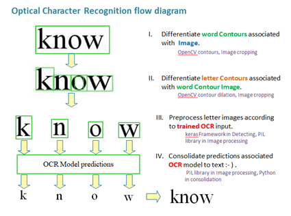
For these programs to work the computer must be able to effectively isolate each character:

Images are a challenging data source because camera resolution, light sources, distance from the subject, and focus can all impact data quality. As a result, the first step in many applications that require computers to extract features from images is to process the image in a way that isolates the important information and standardizes some of the inputs.
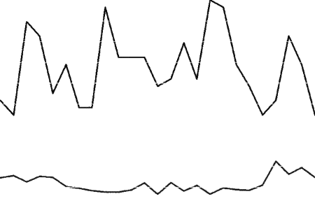
Let’s consider this basic program that allows you to take a picture of a graph, then will generate the underlying data for you. It does this by identifying the trend line, converting it to a pixel grid, then for each horizontal pixel measuring the vertical location of the trend line.
Input image data can be messy, though. So first we need to standardize it to isolate the trend line.
Raw image of a graph:
Step 1: Convert the colored picture to a grayscale version that emphasizes boundaries of graphics.
Step 2: Filter out any data that is below a threshold for opacity or darkness.
Step 3: Convert to a negative view to maximize the contrast of the image.
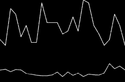
The use of filters in this way is a common first step for models that use images as raw data sources. This will be true for self-driving vehicles that use cameras to collect data streams, or examples from the Digital Humanitarians text that use satellite images to predict the location of damage from a disaster. Next we will look at how these techniques are used to conduct a tree census.
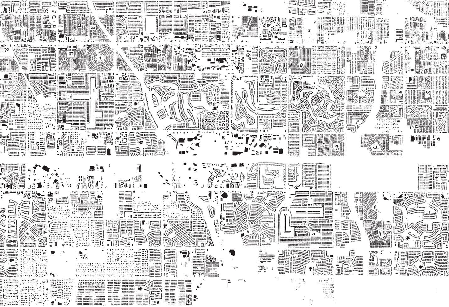
For an interesting urban policy application of this approach, thanks to an program built by Microsoft you can now download a database of every single building in the United States that was built by an AI application that was taught to read satellite images.
Does anyone recognize this community?
 Trees
Trees
Trees are important for cities, but maintaining a robust urban forest is expensive and challenging. “Trees clean the air and water, reduce stormwater floods, improve building energy use, and mitigate climate change, among other things. For every dollar invested in planting, cities see an average $2.25 return on their investment each year.” cite
If we want to decide where to plant trees in our city by bringing a data-driven approach to tree policy, we first need to measure the outcome. “How many trees are in your city? It might seem like a straightforward question, but finding the answer can be a monumental task. New York City’s 2015-2016 tree census, for example, took nearly two years (12,000 hours total) and more than 2,200 volunteers.” cite
Using high-resolution images that can capture a wide spectrum of light, data scientists have designed ways to use public data sources and AI to perform this task. Here is a high-resolution image of Washington DC that has eliminated all of the light except that reflecting off of green objects, i.e. plant life in the city (as opposed to buildings and parking lots):
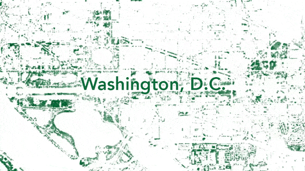
Easy enough, right? But wait! Green patches might be grass, shrubs, or flowers. How does the program know NOT to count these green patches as trees?
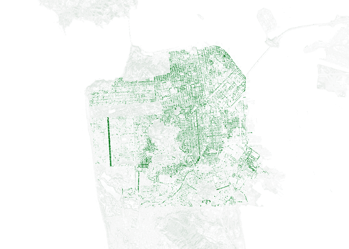
It turns out that trees reflect green light differently than other plants. If you apply the right filters you can further isolate the trees in the image from the rest of the plants. For example, watch the grass in the park disappear:
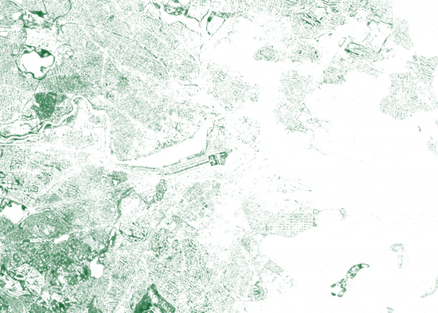
Or eliminate all of the open green spaces in Boston (the grass at the airport is especially vivid):
These techniques allow us to isolate trees from everything else. But we now have another problem - a green island rarely contains a single tree. How can we isolate individual trees from a group of trees in a cluster?
The nice tutorial on tree canopy analysis offers some solutions.
The basic recipe for identifying trees within a cluster is to:
1. Apply a Filter to isolate trees from other elements on the landscape.
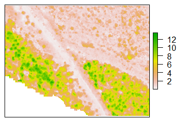
2. Detect Treetops using an algorithm that can predict the height of each pixel in the image.
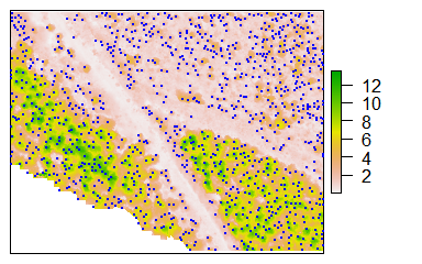
This step returns the geographic coordinates of each tree-top in the cluster so that you can see the tree through the forest.
Note that Lidar uses lasers to enhance digital photographic techniques by including rich measures of light frequency and the ability to triangulate height. Lidar is an expensive technology, but many cities have a database of Lidar images that are open for public use.
3. Model Canopies by using a geometric tesselation algorithm to predict canopy boundaries and create a new spatial file that contains both tree coordinates, heights, and canopy sizes.
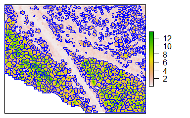
This information would be useful for tracking the number of trees as well as changes in canopies over time.
Faces
Facial recognition software has become accurate and ubiquitous. What features does a computer need in order to recognize a person? How are these features engineered from a two-dimensional image of a face?
Feature Extraction
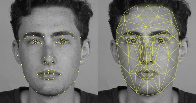
Similar to the programs that read text in images above by identifying text then isolating characters, facial recognition software starts by scanning an image to look for faces. If it finds one it then has a routine to frame the face, then isolate prominent features on the face:
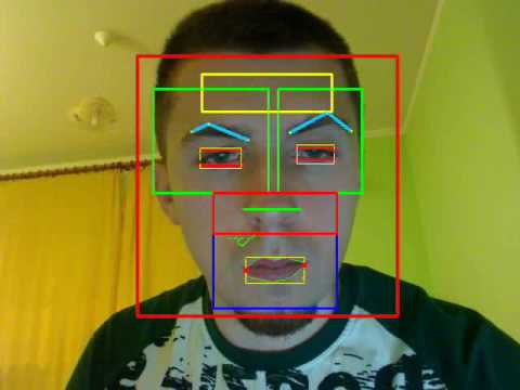
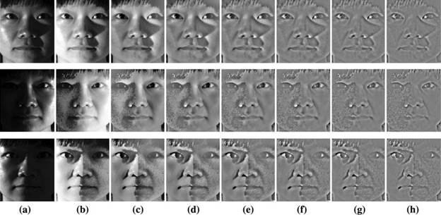
Similar to the hand-writing recognition example, we can apply filters to an image to accentuate specific features. With letters on paper we are trying to maximize the contrast between the ink and the page. With faces, different filters applied to images (or image processing algorithms) will highlight specific facial features.
Once oriented to the face, an algorithm can identify facial landmarks (which is actually similar to how our own brains recognize faces):
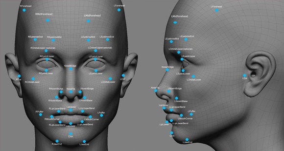
The computer translates the landmark view of a small set of prominent features of a face to a grid model that measures the distance between each feature:
Voila! We now have a format that can be used to generate quantitative variables describing a face. Each line represents a distance between facial landmarks. The length of each line becomes a distinct feature that can be measured and quantified.
You don’t always know the distance from the camera to the face, so you might not be able to predict the actual size of specific features (is my nose big or was the camera just way too close?), but it is easy enough to calculate relative sizes. If you set the distance between the eyes as a measure of one unit, for example, then every other distance on this graph (each line) can be calculated relative to that distance. Thus, you are not identifying individuals based upon the actual size of their noses, but by the relative distances between all features on their face.
There are different ways to accomplish this basic process of creating abstract mathematical models of the face. They all return a list of quantitative features that describe an individual face.
And finally, we compare the measurements from a specific face against measurements in a large database of candidate faces. You can do this quickly because you are working with a few dozen measures (distance between eyes, distance between edges of the mouth, distance between edge of mouth to eye, etc.). You would calculate the difference between the face you are trying to identify, and each face in the database by comparing the length of each line.
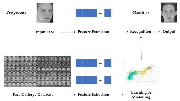
If the total distance between all of the features falls below a threshold, then the faces are flagged as a match to be examined further by a human, or some action is triggered (unlocking your phone or your front door, for example).
Feature Selection
Assuming that the photos are taken in good light with forward-facing subjects and decent resolution cameras, what do you anticipate being a challenge with this process? Facial feature landmarks might vary greatly based upon expressions (or angles of the camera):
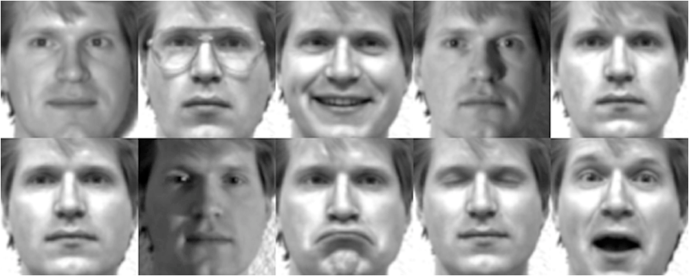
Note that some features, like distance between the eyes and size of the nose, will be static (i.e., reliable measures). Others, like the edges of the mouth or the size of lips, will be highly dependent upon the expression (i.e., low alpha if we think about facial features as latent constructs).
Stated another way, some features convey more information about the unique identity of an individual than others. The feature selection task is to identify which measures will contain the highest signal-to-noise ratios. The algorithms that match faces can also weight certain features more than others to account for expressions.
This paper explores the issue by examining which facial features contain the most information during the recognition task. They do this by examining which features, when changed, render the individual most unrecognizable.
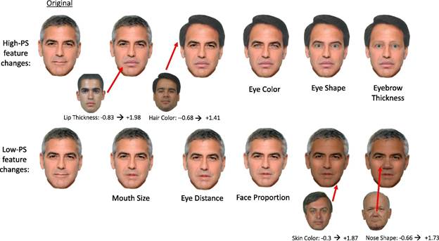
Stated differently, if you omitted the high-salience features from your model like lip thickness, you would see a large drop in correct matches to the database. If you omit low-salience features like mouth size, you experience a lower impact on the accuracy of facial recognition.
This example is meant to give you an intuitive sense of what the computer algorithm might experience as features are “corrupted” in the images and remind you of the importance of the feature selection task.
So, if you are trying to escape the country by crossing a border, which feature would you try to disguise?
LAB QUESTIONS
Part 1: Letters
Assume you have designed a program that can effectively isolate individual characters from an image of a license plate:
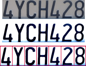
You now want to develop a machine learning model that will accurately identify each character, so you need to develop a set of features that describe the letters so the computer can begin to tell them apart.
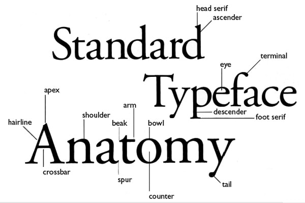
For the lab, list three features of characters that could be reliably derived (“engineered”) from an image of a single letter and used as input data for a predictive model that can read a license plate accurately. Note that fonts used by states might vary, so letters and digits will not be identical.
If you think this sounds challenging, recognize that there are hundreds of potential features (characteristics of the letter). Just look at how many terms hipsters have invented to lovingly diagram their favorite typefaces:
Or spend five minutes with a hand-writing analyst.
It may be helpful for you to start by describing the difference between these letters to a child.
You might start by pondering how someone would distinguish the difference between a lowercase “o” and a lowercase “a”.
How would you describe the difference between a “1” and an “l”?
Between a zero “0” and an upper-case “O”?
Capital “T” versus lower-case “t”?
Part 2: Using Uniforms to Predict Job Title
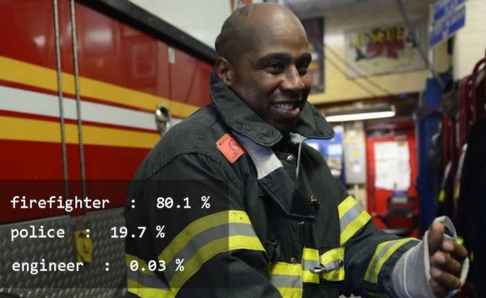
The blog Toward Data Science describes an interesting machine learning application that predicts which category that an object or person belongs to based upon an image. They demonstrate the software by training it to guess people’s career based upon a picture of them at work:
For this tutorial, we have provided a dataset called IdenProf. IdenProf (Identifiable Professionals) is a dataset that contains 11,000 pictures of 10 different professionals that humans can see and recognize their jobs by their mode of dressing.
There are ten professions used in the example:
Chef
Doctor
Engineer
Farmer
Firefighter
Judge
Mechanic
Pilot
Police
Waiter
This dataset is split into 9000 pictures (900 pictures for each profession) to train the artificial intelligence model and 2000 pictures (200 pictures for each profession) to test the performance of the artificial intelligence model as it is training. IdenProf has been properly arranged and made ready for training your artificial intelligence model to recognize professionals by their mode of dressing. For reference purposes, if you are using your own image dataset, you must collect at least 500 pictures for each object or scene you want your artificial intelligence model to recognize.
For the lab, suggest three features of uniforms that might be used to classify images from a profession. Also include a rule statement about how the feature maps the specific profession.
For example:
Rule: If the uniform has stripes on the arms, Prediction the individual will be either a fire fighter or a pilot.
Some more examples:
If the uniform includes a skirt the individual is not a farmer, mechanic, or chef (on the job).
If the uniform is mostly black, the individual will be a judge, pilot, or police officer.
If the uniform is mostly white, the individual will be a chef or a doctor.
If the uniform includes a bow tie, the individual will likely be a waiter (or an engineer?).

Part 3: Home Values
We have focused so far on feature engineering examples that use images as the input data, then extract features based upon models of letter style, tree structure, or the topology of faces. In these instances, we are translating from one data type (an image) to a traditional set of quantitative variables in a spreadsheet format (columns represents variables or features, and rows represent observations).
It is also common to engineer features from an existing dataset, to create new variables from existing variables. For example, population density is a common variable used in urban policy. This variable requires that you have a measure of the population of an administrative unit (number of people in a census tract) and the total geographic area of that unit. Density is then calculated as people per square mile (or whatever unit you use for area).
Population density is often a more useful variable than the raw population because it tells you something about the average distance between individuals in a city. If you are opening a pizza delivery business, for example, the total population of the city does not matter if they are spread out over a large area. You will be more profitable serving a smaller population that is packed into a tight neighborhood than a large suburb which requires long delivery times and high operating costs. Stated differently, population density is a better predictor of the profitability of your new business.
The urban policy research group, Urban Spatial, offers a nice example of this in a model they created to predict gentrification of census tracts using historic census data.
They describe several features that they engineer for the model. Similar to other community change models we have examined, they measure characteristics of housing in census tracts to predict how each might change over time.
One thing they do differently from previous models, however, is use information about home value contagion. When home values rise in an adjacent census tract it increases the likelihood that home values rise in my census tract. This type of relationship is called a spatial correlation. This might occur because people that are looking to buy in a specific neighborhood might be priced out by rising costs in that neighborhood, so they instead purchase a home in an adjacent neighborhood. Higher demand from the spill-over will drive up prices.
Similarly, a drop in prices in a neighborhood can have a contagion effect if buyers looking at purchasing in an adjacent neighborhood get nervous about falling prices and look elsewhere, thus reducing the demand and lowering prices, resulting in a self-fulling prophesy in some instances.
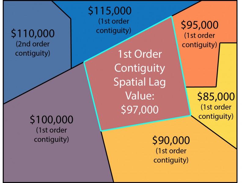
To model these processes, you need to take into account information about neighboring communities. The paper Urban Spatial explains how they create (engineer) two variables (features) for their model.
One variable is created by calculating the average value of homes in all of the surrounding census tracts. Only those census tracts that are contiguous to your own (they share a border) are included. So, the census tract in the top left corner is excluded in the calculation, for example:
The second variable was created after recognizing that the average value of surrounding homes might not be the best predictor of change. Rather, homeowners typically want to move into hot neighborhoods that have nice amenities and cool people. Since everyone wants to move there, though, these neighborhoods quickly become saturated and overpriced, and buyers spill over into nearby neighborhoods.
They identified all of the census tracts in the top 5th of the data (the top 20% of tracts based upon home values) and categorize them as highly-desirable tracts. They then calculate the distance from each tract in the dataset to the nearest highly-desirable tract:
If we are predicting home values for a tract in 2010, the value in 2000 will provide a reference point for where home values start but will not tell you much about whether you expect them to be rising or falling. The value of neighboring tracts, however, is a good predictor (if adjacent tracts have more expensive homes, prices are likely to rise, if they have cheaper homes, prices will likely fall). And the distance to the closest “hot” neighborhood in 2000 will provide a different type of information about possible trends. The two variables that explain trends are both second-order variables that are created from the raw census data.
For the Lab: recall that in the previous lab you were required to identify a neighborhood or metropolitan feature that impacts home values (for example, every time a Starbucks opens in a new neighborhood home values increase by 0.5%).
Using the feature that you identified in Lab 2 (or another you may need to choose), explain how you would “engineer” it by answering the following questions. You are NOT allowed to use a metric that is already an existing census variable and requires no engineering (i.e., calculation).
1. What is your unit of analysis? Census tract, zip code, city, etc.
Some variables are better at a very local scale (crimes tend to impact prices on surrounding blocks but not much further), whereas others are only meaningful at a metro or regional scale (i.e., activity of regional airports).
2. What type of data do you need to calculate the variable?
What measures are included in your formula? For example, if a new Starbucks impacts home values, you would measure the distance to it for each home. You would need a database of Starbucks in your city with their locations.
3. What is the process or formula you would follow to create the variable?
Write out instructions for calculating your metric in a way that a data engineer could implement. For example, to calculate the distance to the nearest Starbucks:
Identify the location of each home in the dataset.
Identify the nearest Starbucks.
Calculate the distance between the two points.
Note! These instructions are not specific enough because you can easily calculate the Euclidian distance between two points on a map with a formula, but how often do you travel in a straight line to a destination? Maybe a travel distance time derived from Google maps might be a better metric? Or maybe travel time, rather than distance? Are you assuming people are walking, driving, or taking public transit?
4. How reliable will your measure be?
Using your knowledge about instrument development, do you feel like your new variable will accurately reflect the true underlying latent construct you are trying to measure? For example, using the programs described in the lab, I could fairly accurately measure the total tree canopy cover for a specific neighborhood (the average is about 20% coverage in most cities). If I were trying to create a hipster scale to measure how cool a neighborhood is by identifying how many local menus include craft beer, my scale might be less reliable (largely because craft beer is mainstream, not cool enough).
Looking Ahead
The goal behind the design of the last three labs was (1) to encourage you to think about how the data that we use every day and that has a big impact on our lives is created, and (2) to demystify machine learning and artificial intelligence. These exercises were designed to give you insight into the black box of predictive analytics, remote sensors, and artificial intelligence.
You do not need to know how to build a car from scratch to be a good driver. Similarly, you do not need to be a data scientist to incorporate these new tools into your future career. Your job as a future analyst or manager, for example, may be to determine whether automation or a predictive model would add value to your organization. If so, you can hire an expert to build the models for you.
That said, a little bit of vocabulary will help you write a call for proposals, interview potential firms, and manage the process along the way. The processes of feature selection and measurement can be challenging for an outside expert that doesn’t intimately understand your program. You can add a lot of value by collaborating with the experts during the process to identify latent constructs, select features that are important to the question at hand, and discussing how the data may need to be engineered for analysis and/or modeling.